
Làm sao để tính tổng hoặc đếm dữ liệu dựa trên màu sắc của ô hoặc màu sắc của ký tự trên bảng tính ? Nếu bạn đang thắc mắc câu hỏi này và chưa tìm được giải pháp phù hợp hãy tham khảo bài viết sau đây. Trong bài viết này, chúng tôi sẽ hướng dẫn bạn cách ứng dụng hàm màu sắc trong Excel để xử lý dữ liệu hiệu quả hơn, cùng theo dõi nhé!
Table of Contents
Tìm hiểu cơ bản về hàm màu sắc trong Excel
Trong thực tế, COLOR không phải là một hàm có sẵn trong Excel, nó là một hàm UDF - user defined function do người dùng tự viết ra thông qua VBA. Hàm này có thể giúp bạn tính toán và đếm dữ liệu trên các ô trong bảng tính thông qua màu sắc. Để cài đặt hàm này, bạn cần thực hiện như sau:
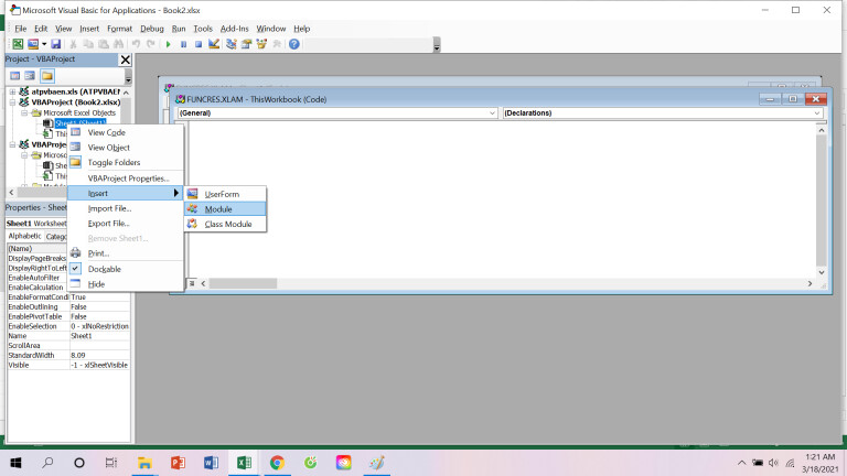
Bước 1: Mở giao diện VBA (visual basic editor) bằng phím tắt Alt + F11, sau đó truy cập vào Project → VBA Project → Insert → Module
Bước 2: Trên bảng tính mới được mở, bạn cần nhập dòng code sau đây:
Function GetCellColor(xlRange As Range)
Dim indRow, indColumn As Long
Dim arResults()
Application.Volatile
If xlRange Is Nothing Then
Set xlRange = Application.ThisCell
End If
If xlRange.Count > 1 Then
ReDim arResults(1 To xlRange.Rows.Count, 1 To xlRange.Columns.Count)
For indRow = 1 To xlRange.Rows.Count
For indColumn = 1 To xlRange.Columns.Count
arResults(indRow, indColumn) = xlRange(indRow, indColumn).Interior.Color
Next
Next
GetCellColor = arResults
Else
GetCellColor = xlRange.Interior.Color
End If
End Function
Function GetCellFontColor(xlRange As Range)
Dim indRow, indColumn As Long
Dim arResults()
Application.Volatile
If xlRange Is Nothing Then
Set xlRange = Application.ThisCell
End If
If xlRange.Count > 1 Then
ReDim arResults(1 To xlRange.Rows.Count, 1 To xlRange.Columns.Count)
For indRow = 1 To xlRange.Rows.Count
For indColumn = 1 To xlRange.Columns.Count
arResults(indRow, indColumn) = xlRange(indRow, indColumn).Font.Color
Next
Next
GetCellFontColor = arResults
Else
GetCellFontColor = xlRange.Font.Color
End If
End Function
Function CountCellsByColor(rData As Range, cellRefColor As Range) As Long
Dim indRefColor As Long
Dim cellCurrent As Range
Dim cntRes As Long
Application.Volatile
cntRes = 0
indRefColor = cellRefColor.Cells(1, 1).Interior.Color
For Each cellCurrent In rData
If indRefColor = cellCurrent.Interior.Color Then
cntRes = cntRes + 1
End If
Next cellCurrent
CountCellsByColor = cntRes
End Function
Function SumCellsByColor(rData As Range, cellRefColor As Range)
Dim indRefColor As Long
Dim cellCurrent As Range
Dim sumRes
Application.Volatile
sumRes = 0
indRefColor = cellRefColor.Cells(1, 1).Interior.Color
For Each cellCurrent In rData
If indRefColor = cellCurrent.Interior.Color Then
sumRes = WorksheetFunction.Sum(cellCurrent, sumRes)
End If
Next cellCurrent
SumCellsByColor = sumRes
End Function
Function CountCellsByFontColor(rData As Range, cellRefColor As Range) As Long
Dim indRefColor As Long
Dim cellCurrent As Range
Dim cntRes As Long
Application.Volatile
cntRes = 0
indRefColor = cellRefColor.Cells(1, 1).Font.Color
For Each cellCurrent In rData
If indRefColor = cellCurrent.Font.Color Then
cntRes = cntRes + 1
End If
Next cellCurrent
CountCellsByFontColor = cntRes
End Function
Function SumCellsByFontColor(rData As Range, cellRefColor As Range)
Dim indRefColor As Long
Dim cellCurrent As Range
Dim sumRes
Application.Volatile
sumRes = 0
indRefColor = cellRefColor.Cells(1, 1).Font.Color
For Each cellCurrent In rData
If indRefColor = cellCurrent.Font.Color Then
sumRes = WorksheetFunction.Sum(cellCurrent, sumRes)
End If
Next cellCurrent
SumCellsByFontColor = sumRes
End Function
Bước 3: Để hoàn tất bạn lưu bảng tính mới với tên “Excel Macro - Enabled Workbook.xlsm” để hoàn tất.
Một số ứng dụng của hàm COLOR trong Excel
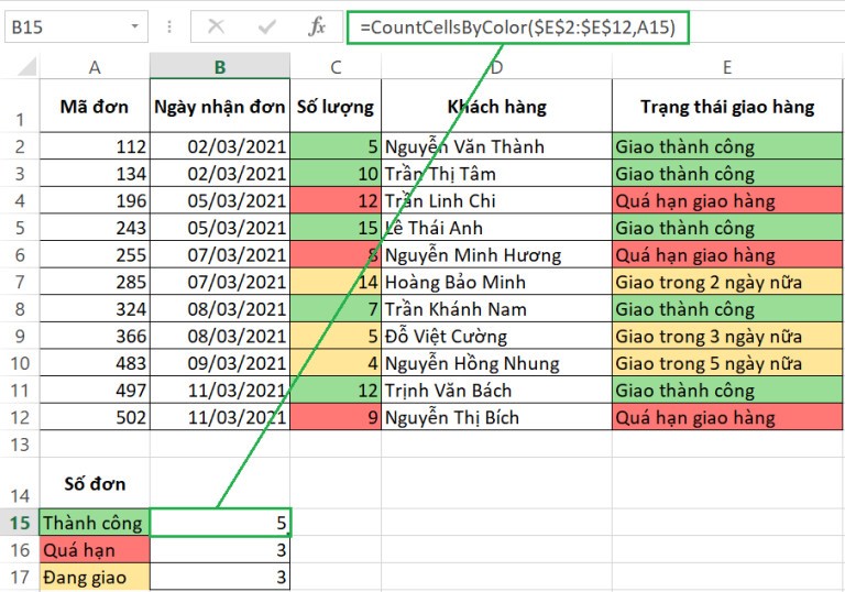
Để thực hành sử dụng hàm COLOR đúng, chúng ta sẽ phân tích các ứng dụng của hàm này trong ví dụ sau đây. Chúng ta có bảng tính (xem ví dụ ở ảnh minh họa) thể hiện trạng thái giao hàng của công ty chuyển phát hàng hóa. Trong đó cột E thể hiện trạng thái giao hàng với màu sắc tương ứng, màu xanh lục thể hiện “Giao hàng thành công”, màu đỏ thể hiện “Quá hạn giao hàng”, màu vàng thể hiện trạng thái “Giao hàng trong xx ngày”. Yêu cầu cần đếm trạng thái giao hàng theo màu sắc hoặc tính tổng số đơn hàng theo màu sắc.
Để đếm trạng thái giao hàng, bạn cần sử dụng hàm COLOR theo công thức:
=CountCellsByColor(range, color code) với range là phạm vi dữ liệu cần đếm, color code đại diện cho màu dữ liệu cần đếm.
Trong ví dụ trên, để đếm số trạng thái giao hàng thành công bạn cần nhập công thức:
=CountCellsByColor($E$2:$E$12,A15) với E2:E12 là phạm vi dữ liệu, A15 là đại diện màu sắc cần đếm, $ dùng để cố định dữ liệu, kết quả được thể hiện ở ảnh dưới đây.
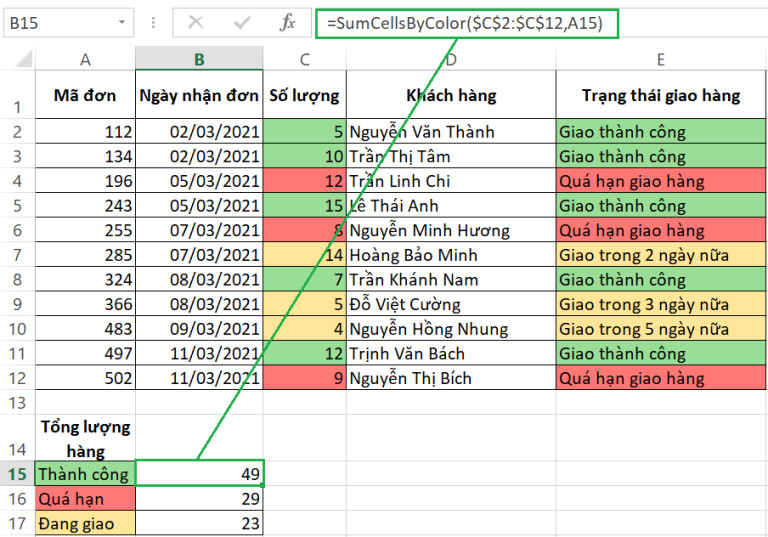
Để tính tổng số lượng hàng hóa trong cột C theo màu sắc, bạn cần sử dụng công thức:
=SumCellsByColor(range, color code) với với range là phạm vi dữ liệu cần đếm, color code đại diện cho màu dữ liệu cần tính.
Cụ thể với ví dụ này cần nhập công thức: =SumCellsByColor($C$2:$C$12,A15) với C2:C12 là phạm vi dữ liệu, A15 đại diện cho màu sắc cần đếm, kết quả được minh họa ở hình sau:
Trên đây là bài viết hướng dẫn sử dụng hàm màu sắc trong Excel để đếm và tính toán dữ liệu. Mong rằng, sau khi tham khảo bài viết, bạn đọc đã hiểu hơn về hàm COLOR và ứng dụng tốt hàm này trong quá trình xử lý dữ liệu của mình. Hãy theo dõi blog của chúng tôi để tìm hiểu thêm nhiều mẹo hay về Excel trong thời gian tới bạn nhé!
Tìm hiểu các hàm hữu ích khác:
- Hàm find trong excel
- Hàm index trong excel
- Hàm lấy ký tự có điều kiện trong excel
- Hàm lọc dữ liệu có điều kiện trong excel
- Hàm match trong excel


